Developer Manual
This document aims to provide the reader with the necessary information to be able to extend or customize dtControl. We first give an overview of the general software architecture of the tool. Then, we show how support for controllers in new file formats can be added, explain the inner workings of the decision tree (DT) learning component, and explore how dtControl could be extended with new output formats.
Overview
dtControl is written entirely in Python and makes use of both the numpy and scikit-learn packages for data representation and manipulation. A basic familiarity with this programming environment is assumed throughout this manual. More information on dependencies can be found in the provided readme and setup.py files.
An overview of the software architecture of dtControl is given in the following UML component diagram:
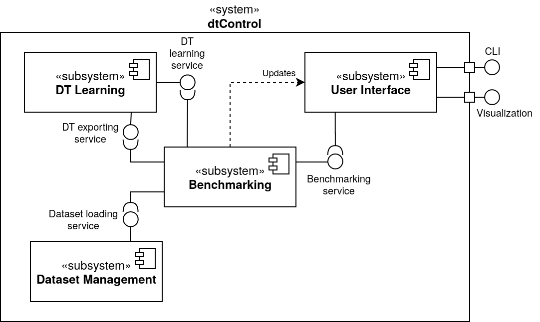
The heart of the tool is formed by the DT Learning subsystem, which is responsible for the actual decision tree algorithms and representation. It provides all of the different options for training DTs and can export the learned trees in the DOT and C format.
To make the DT learning itself independent of any verification tool, the Dataset Management has been extracted into a separate subsystem, which mainly provides functionality for loading and converting controllers from many different sources such as SCOTS, Uppaal Stratego, and PRISM.
The Benchmarking component is responsible for running a set of different given DT learning configurations on a number of specified controllers. It thus uses both the functionality provided by the Dataset Management and the DT Learning subsystems.
Finally, the User Interface serves as the main entry point for user interaction with the tool, in the form of a CLI. The constructed HTML files with benchmark statistics also belong to the user interface.
Supporting New File Formats
dtControl currently supports the file formats generated by the the tools SCOTS, Uppaal Stratego, and PRISM. There are two ways to make the tool work with other formats, as described in the following.
The CSV format
The first option is to convert the new file format to a custom CSV format that dtControl also supports. We now describe the specification of the custom CSV format.
The first two lines of the file are reserved for metadata. The first line must always reflect whether the controller is permissive (non-deterministic) or non-permissive (deterministic). This is done using either of the following lines:
#PERMISSIVE
or:
#NON-PERMISSIVE
The second line must reflect the number of state variables (or the state dimension) and the number of control input variables (or the input dimension). This line looks as follows:
#BEGIN N M
where N is the state dimension and M is the input dimension.
Every line after the 2nd line lists the state action/input pairs as a comma separated list:
x1,x2,...,xN,y1,y2,...,yM
if the controller prescribes the action (y1,y2,...,yM) for the state (x1,x2,...,xN). If the state allows more actions, for example, (y1’,y2’,...,yM’), then this should be described on a new line:
x1,x2,...,xN,y1,y2,...,yM
x1,x2,...,xN,y1’,y2’,...,yM’
An excerpt of the 10rooms.scs controller written in this CSV format would look as follows:
#PERMISSIVE
#BEGIN 10 2
18.75,20.0,18.75,18.75,20.0,18.75,18.75,18.75,18.75,18.75,1.0,1.0
20.0,20.0,18.75,18.75,20.0,18.75,18.75,18.75,18.75,18.75,1.0,1.0
21.25,20.0,18.75,18.75,20.0,18.75,18.75,18.75,18.75,18.75,1.0,1.0
18.75,21.25,18.75,18.75,20.0,18.75,18.75,18.75,18.75,18.75,0.0,1.0
18.75,21.25,18.75,18.75,20.0,18.75,18.75,18.75,18.75,18.75,0.5,1.0
18.75,21.25,18.75,18.75,20.0,18.75,18.75,18.75,18.75,18.75,1.0,1.0
20.0,21.25,18.75,18.75,20.0,18.75,18.75,18.75,18.75,18.75,0.0,1.0
dtControl will automatically look for files with a .csv extension and parse them with the assumption that they follow this format.
Implementing a new dataset loader: The dataset management subsystem
Additionally, it is also possible to integrate the new file format natively into dtControl by providing a dataset loader. For this, we will take a closer look at the Dataset Management subsystem.
An overview of the subsystem is given in the following UML class diagram:
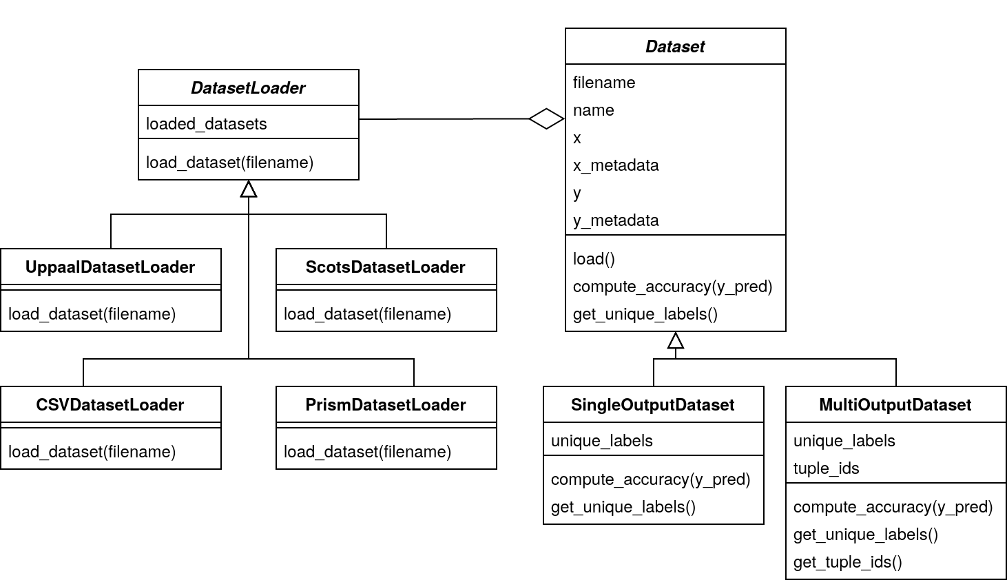
The Dataset class is what the DT learning algorithm needs to train a decision tree. A Dataset can either be a SingleOutputDataset if it only has a single control input, or a MultiOutputDataset if there are multiple control inputs.
Note
Since the code focuses on the decision trees themselves, it refers to the output of those trees, which is the same as the action produced by the controller, i.e. the control input.
Its most important properties are detailed in the following:
xis a simple NumPy array containing the values of the state variables. It has dimension #number of states in the controller ✕ #number of state variables.x_metadatais a dictionary containing metadata about the arrayx. For instance, it contains the names of the variables (if available), the minimum and maximum value inx, and indicates which columns ofxare categorical.yis a NumPy array containing the actions that can be performed for every state. Its format differs, depending on whether the dataset is single- or multi-output:In the case of single-output datasets,
yis a two-dimensional array where each row contains all (non-deterministic) actions that can be performed at the corresponding row ofx. Instead of the actual (possibly) floating point values, we use integer indices representing those values throughout the code; the mapping of indices to the actual values can be found indataset.index_to_value. Since NumPy usually cannot deal with rows of different sizes, but we have varying numbers of possible actions, some rows have to be filled with-1s. These-1s have to be ignored during tree construction.In the case of multi-output datasets,
yis a three-dimensional array whose first dimension (or axis) corresponds to the different control inputs. Thus, there is a two-dimensional array for each control-input, which exactly matches the structure outlined above. The DT learning algorithms implemented so far all convert from this representation to the tuple ID representation in which every action(y1,y2,...,yM)is replaced with a single tuple id. The methodget_tuple_ids()returns an array of labels in this tuple ID representation, which again matches the structure of theyarray in the single-output case.
y_metadatais a dictionary containing metadata about the arrayy. Similarly tox_metadata, it indicates which columns ofyare categorical outputs, and provides some other information such as the minimum and maximum value iny.
The Dataset class provides some auxiliary functionality for the DT learning algorithm, such as compute_accuracy(y_pred) and get_unique_labels(), as well as a load() method that uses a DatasetLoader to actually load the dataset from a file into the internal NumPy representation.
It is this DatasetLoader class that needs to be extended in order to add support for a new file format to dtControl. A new DatasetLoader must provide exactly one method: _load_dataset() parses a file in the new format and returns the tuple (x, x_metadata, y, y_metadata, index_to_value) which corresponds to the attributes of a Dataset as outlined above.
The new dataset loader can be registered in the extension_to_loader dictionary in the Dataset class. Now, if dtControl encounters a file with an extension of the new file format, it will attempt to load it using the registered loader.
You may find inspiration for writing your own dataset loader in some of the already existing ones such as the UppaalDatasetLoader or the relatively simple PrismDatasetLoader. However, they are very specific to their respective file format.
Extending dtControl with new algorithms: The decision tree learning subsystem
dtControl already supports a wide variety of decision tree construction algorithms. Furthermore, the tool can readily be extended with new algorithms, as we will see in this section.
We again start with a UML diagram of the DT learning subsystem. In order to keep it as flexible as possible, we use a composition-based approach that makes heavy use of interfaces. This has the advantage that you only need to develop against a specific interface if you want to only extend a part of the DT learning algorithm. For instance, if you want to add a new impurity measure, you just have to provide an implementation of the ImpurityMeasure interface and your code will immediately integrate with the rest of the learning algorithm.

As can be seen, the heart of the component is the DecisionTree class, which offers the core methods one would expect:
fit(dataset)constructs a decision tree for a dataset.predict(dataset)returns a list of control inputs predicted for a dataset.get_stats()returns the statistics to be displayed in the benchmark results as a dictionary. This will mainly include the number of nodes and potentially some algorithm-specific statistics.print_dot()saves a representation of the decision tree in the DOT format.print_c()exports the decision tree to a C-file as a chain of if-else statements.print_vhdl()returns the corresponding vhdl code.toJSON()converts theDecisionTreeobject to aJSONdictionary.
Most of these methods simply delegate to the root object of type Node, which implements the actual decision tree data structure. It has mostly the same attributes as a DecisionTree, as well as some statistics and either a list of children or a label. Depending on the dataset and algorithm, a label can be one of the following:
A single integer (that appears in the
index_to_valuedictionary) corresponding to a single actionA single tuple of integers corresponding to a single action with multiple outputs
A list of integers corresponding to multiple possible actions
A list of tuples corresponding to multiple possible actions with multiple outputs
We now examine the most important interfaces in detail.
Splitting strategies
A SplittingStrategy provides the method find_split(dataset, impurity_measure), which returns the best predicate of a certain type, given a dataset and an impurity measure. For instance, the AxisAlignedSplittingStrategy searches through all possible axis-aligned splits for the given dataset and returns the one with lowest impurity. Additionally, if several different splitting strategies are in use, the user can assign an individual priority to the strategies. The priority is later taken into account when calculating the impurity of the predicate \(p_i\). The new impurity (with priority in \((0,1]\)) is calculated as the following:
Note
The default value of priority is 1. By assigning the exclusive priority of 0, the user can specify a FallbackStrategy, a strategy which should only be used if all other strategies fail.
The returned predicate is of type Split and must provide the following methods:
predict(features)returns an index into thechildrenlist of aNodecorresponding to the child that should be picked for the given NumPy array of features.get_masks(dataset)returns a list of NumPy masks indicating how the dataset is split. A mask is just a one-dimensional array of boolean values with a length oflen(dataset). A value ofTruein the jth row of the ith mask indicates that the jth row indataset.xbelongs to the ith sub-dataset created by the split.print_dot()returns the string that should be put in the node in the DOT format.print_c()returns the string that should be put in the corresponding if-statement in the C code.print_vhdl()returns the string that corresponds to vhdl code.to_json_dict()converts theSplitobject to aJSONdictionary.
The simplest example of a Split is probably the AxisAlignedSplit.
Impurity measures
An ImpurityMeasure needs to provide the calculate_impurity(dataset, split) method, which simply returns a float indicating the impurity. There are two types of impurity measures:
MultiLabelImpurityMeasuresdirectly compute the impurity from the nondeterministic labels. Examples includeMultiLabelEntropyandMultiLabelGiniIndex.DeterminizingImpurityMeasurescorrespond mostly to the traditional impurity measures known from decision trees in machine learning. Examples includeEntropyandGiniIndex. These impurity measures are called determinizing since they don’t directly work on the nondeterministic labels. Instead, the use aDeterminizerthat first converts the labels to a new representation.By default, the
LabelPowersetDeterminizeris used, which treats every combination of possible labels as a unique label and thus preserves all of the nondeterminism present in the original controller. Other options are for example theMaxFreqDeterminizer, which implements the maximum frequency determinization technique. Determinizers can either be applied before or after splitting, as indicated by theis_pre_split()method.
Determinization
The final ingredient of the DT learning algorithm - determinization - is mainly controlled by the early_stopping attribute of a DecisionTree. If it is set to True, early stopping is performed and the resulting DT is thus (possibly) smaller and more deterministic. This parameter should always be enabled if impurity measures that make use of determinization are used, such as the MultiLabelEntropy or any DeterminizingImpurityMeasure with the MaxFreqDeterminizer.
Instead, one can also choose to determinize the controller itself before DT learning with a LabelPreProcessor, such as the NormPreProcessor. For this, the methods preprocess_single_output(dataset) and preprocess_multi_output(dataset) that return a NumPy array of determinized labels must be provided.
Finally, decision trees can also be post-processed by a PostProcessingMethod such as safe pruning. The most important method of the class is run(), which runs the post-processing technique on its classifier, transforming the decision tree.
Supporting New Output Formats
As shown above, the core decision tree data structure is implemented in the DecisionTree and Node classes. These classes also offer functionality for DOT and C printing.
To add a new output format to dtControl, one thus would have to provide new exporting methods in the DecisionTree and Node classes. Furthermore, the BenchmarkSuite would have to be adapted to export the tree to the new output format once a DT has been constructed.
Predicate Parser
The PredicateParser class provides all core methods to process predicates, provided by the user. The core methods are called:
get_domain_knowledge()parses a whole file, containing domain knowledge.get_predicate()parses a wholetxtfile, containing predicates.parse_single_predicate(single_predicate)parses a single predicate, provided as String.parse_user_string(user_input)parses a string, which contains more than one predicate. Typically used when working with the frontend.parse_user_interval(interval)parses a single interval, provided as String and returns a SymPy interval.
The final returned predicates of the PredicateParser are of type Richer Domain Split.
Richer Domain Split
The RicherDomainSplit class is used to represent predicates given by the user. Additionally to the already mentioned methods of the Split class, (which can be found in Splitting strategies) it provides following attributes:

For demonstration purposes, consider an example user given predicate of following structure:
c_1 * x_1 - c_2 + x_2 <= 0; x_2 in {1,2,3}; c_1 in (-inf, inf); c_2 in {1,2,3};
column_intervalis a dict storing all given column intervals. Key:Sympy SymbolValue:Sympy Interval. In the running example:column_interval = {x_1:(-Inf,Inf), x_2:{1,2,3}}
coef_intervalis a dict storing all given coefficient intervals. Key:Sympy SymbolValue:Sympy Interval. In the running example:coef_interval = {c_1:(-Inf,Inf), c_2:{1,2,3}}
termis storing the term asSympyexpression. In the running example:term = c_1 * x_1 - c_2 + x_2
relationis aStringcontaining the relation. In the running example:relation = "<="
coef_assignmentis by defaultNone. It will be determined insidefit()and stores a list containing substitution tuples of structure(Sympy Symbol, Value). In the running example:coef_assignment = [(c_1,-8.23), (c_2,2)]
idis a unique uuid to identify a RicherDomainSplit object.
Note
Every symbol without a specific defined Interval will be assigned to the interval: (-Inf, Inf).
Additionally we provide following methods:
get_fixed_coef_combinations()returns a list of fixed coefficients. In the running example:[ [('c_1', 1), ('c_2', -3)], [('c_1', 1), ('c_2', -1)], [('c_1', 2), ('c_2', -3)], [('c_1', 2), ('c_2', -1)], [('c_1', 3), ('c_2', -3)], [('c_1', 3), ('c_2', -1)] ]
contains_unfixed_coefs()returns a boolean if the predicate contains unfixed coefficients. In the running example:false.fit(fixed_coefs, x, y, method)computes the best fit according to the chosenmethod. Available methods are ‘lm’, ‘trf’, ‘dogbox’ or ‘optimized’, which utilizes as often as possible the Levenberg-Marquardt strategy. Only in the edge case where the number of data points is less than the number of parameters the Trust Region Reflective Approach will be used.check_valid_column_reference(x)checks whether the used column reference index is represented in the datasetxor not. In the running example, the function returnstrueif the dataset has at least 3 columns.check_data_in_column_interval(x)checks if the column intervals contain all the values of the datasetx. In the running example, the function returnstrueif all values of the third column are in{1,2,3}.check_offset(offset)compares the offset with the relation to 0. In the running example, the function comparesOffset <= 0.