User Manual

This document equips the user with the information necessary to use dtControl and run the various decision tree learning algorithms implemented in it.

Capabilities

dtControl is a tool to represent controllers using decision trees. It uses decision tree learning to achieve this. The 5-minute video above gives a quick introduction to why and how one may benefit from using dtControl.

The decision tree algorithm running inside dtControl is highly configurable. You may choose to represent a determinized controller, allow for more expressible decision predicates or even tune the heuristic used to pick the best predicate. See Presets and configuration files for more details.

While dtControl achieves best results with permissive or non-deterministic controllers with determinization enabled, it can also be used with deterministic controllers. However empirical results with such controllers are not as significant as with non-deterministic controllers.

Getting Started

A quick start installation guide is available in the README. In this section, we elaborate a little more on the installation process.

Installation

Getting dtControl from the Python Package Index (PyPI) is the recommended way to install it. Before running the pip install command, we recommend creating a virtual environment so that dependencies of dtControl do not conflict with any other packages already installed on your system. The official Python documentation for creating virtual environments may help you set it up. However, we provide the most essential information here.

Once you have a recent version of Python 3 installed, you may run:

$ python3 -m venv venv

to create the virtual environment in a folder called venv located in your current directory. You can enter the virtual environment by running:

$ source venv/bin/activate

Typically, your shell might indicate that the virtual environment is activated by changing the prompt symbol $ to something like (venv) $. You can now proceed with installing dtControl from PyPI using pip:

(venv) $ pip install dtcontrol

Note

In case you want to get the development version of dtControl, you could instead run:

(venv) $ pip install git+https://gitlab.lrz.de/i7/dtcontrol.git

Once the dtControl package is installed, the command line interface can be accessed using the dtcontrol command. Try running:

(venv) $ dtcontrol -h

If your installation has run successfully, you will now see the help page detailing the usage and arguments.:

usage: dtcontrol [-h] [-v] [--input INPUT [INPUT ...]] [--output OUTPUT] [--benchmark-file FILENAME] [--config CONFIGFILE] [--use-preset USE_PRESET [USE_PRESET ...]] [--rerun]
              [--timeout TIMEOUT]
              {preset,clean} ...

 Scroll to the end of the help message for Quick Start.

 optional arguments:
   -h, --help            show this help message and exit
   -v, --version         show program's version number and exit

 input/output:
   --input INPUT [INPUT ...], -i INPUT [INPUT ...]
                         The input switch takes in one or more space separated file names or a folder name which contains valid controllers (.scs, .dump or .csv)
   --output OUTPUT, -o OUTPUT
                         The output switch takes in a path to a folder where the constructed controller representation would be saved (c and dot)
   --benchmark-file FILENAME, -b FILENAME
                         Saves statistics pertaining the construction of the decision trees and their sizes into a JSON file, and additionally allows to view it via an HTML file.

 run configurations:
   --config CONFIGFILE, -c CONFIGFILE
                         Specify location of a YAML file containing run configurarions. Use along with the --use-preset switch. More details in the User Manual.
   --use-preset USE_PRESET [USE_PRESET ...], -p USE_PRESET [USE_PRESET ...]
                         Run one or more presets defined in the CONFIGFILE. If the --config switch has not been used, then presets are chosen from the system-level configuration file.
                         Special parameters for this switch include 'all', 'all-user', 'all-system'. Refer the User Manual for more details.
   --rerun, -r           Rerun the experiment for all input-method combinations. Overrides the default behaviour of not running benchmarks for combinations which are already present in
                         the benchmark file.
   --timeout TIMEOUT, -t TIMEOUT
                         Sets a timeout for each method. Can be specified in seconds, minutes or hours (eg. 300s, 7m or 3h)

 other commands:
   {preset,clean}        Run 'dtcontrol COMMAND --help' to see command specific help

 Examples:
 Create a file storing run configurations
     dtcontrol preset --sample > user-config.yml

 Display all presets available with dtcontrol
     dtcontrol preset --config user-config.yml --list

 Run the 'my-config' preset on the SCOTS model located at 'examples/cps/cartpole.scs'
     dtcontrol --input examples/cps/cartpole.scs --config user-config.yml --use-preset my-config

Input format

Supported tools

dtControl currently supports the file formats generated by the tools SCOTS, Uppaal Stratego, and PRISM. To see how to add suppport for new file formats to dtControl, refer to the Developer Manual.

SCOTS and Uppaal output .scs and .dump files, respectively, as the result of a controller synthesis process. These can directly be specified as input to dtControl.

For PRISM, dtControl expects a strategy file that maps state indices to actions and a states file that maps state indices to the corresponding values of state variables. These files can be generated by PRISM with the following options:

prism firewire_abst.nm liveness_abst.pctl -const 'delay=50,fast=0.5000' -prop 1 -explicit -exportstrat 'firewire_abst.prism:type=actions' -exportstates 'firewire_abst_states.prism'

It is important that both files have a .prism extension and the states file has the same name as the actions file with an _states suffix.

It is also possible to run dtControl on all controllers in a given folder; the tool then simply looks for all files with one of the above extensions.

Specifying metadata

While dtControl tries to obtain as much information as possible from the controller directly, it is sometimes necessary to provide additional metadata to the tool. For example, dtControl cannot know which variables in the controller are categorical, which is necessary for some of the specialized algorithms. It is also possible to specify names, e.g. for variables, which are used in the DOT output.

This metadata can be given in a JSON file named controller_name_config.json (where controller_name must match the name of the controller file), which allows to set the following options:

• x_column_types is a dictionary with two entries, numeric and categorical. These entries are lists with indices specifying which variables are numeric or categorical, respectively.

• y_column_types provides the same information for the output variables.

• x_column_names is a list of variable names.

• x_category_names is a dictionary with one entry for every categorical variable (as specified in x_column_types[categorical]). This entry can either be an index or a name from x_column_names and maps to a list of category names for the variable. For instance, an entry of the form "color": ["red", "green", "blue"] would mean that a 0 in the color variable stands for red, a 1 means green, and a 2 denotes blue.

• y_category_names gives the same information for the output variables.

If any of the options in the metadata are not set, dtControl tries to fall back to reasonable defaults, such as x[i] for the column names or just integers i for the category names. By default, all variables are treated as numeric.

An example is given in form of the configuration file for the firewire_abst.prism case study:

{
  "x_column_types": {
    "numeric": [
      0
    ],
    "categorical": [
      1
    ]
  },
  "x_column_names": [
    "clock",
    "state"
  ],
  "x_category_names": {
    "state": [
      "start_start",
      "fast_start",
      "start_fast",
      "start_slow",
      "slow_start",
      "fast_fast",
      "fast_slow",
      "slow_fast",
      "slow_slow"
    ]
  }
}

This configuration provides the information that the two variables are clock and state, the first of which is numeric and the second of which is categorical. Furthermore, a state of 0 corresponds to start_start, a state of 1 to fast_start, and so on. Note that, for PRISM models, dtControl automatically parses the names of the actions and it is thus not necessary to provide a y_category_names entry.

The command-line interface

This section shows how to configure and run dtControl. For this purpose, we assume that you have an examples folder in your current directory containing cartpole.scs. You can choose to download all of our examples from our Gitlab repository via this zip archive or using git. Extract the contents of the archive into a folder called examples and unzip cartpole.scs.zip. Alternatively, you can run the following commands:

$ mkdir -p examples && cd examples
$ wget -P examples/cps https://gitlab.lrz.de/i7/dtcontrol-examples/-/raw/master/cps/cartpole.scs.zip
$ unzip -d ./examples/cps ./examples/cps/cartpole.scs.zip

Next, activate the virtual environment you installed dtControl in:

$ source venv/bin/activate

Running your first command

Finally, you can run dtControl with the default parameters on the cartpole example (cartpole.scs), use the following command:

(venv) $ dtcontrol --input examples/cps/cartpole.scs

This will produce some new files and folders in the current folder:

decision_trees
|-- default
|   `-- cartpole
|       |-- default.c
|       |-- default.dot
benchmark.json
benchmark.html

Open benchmark.html in your favourite browser to view a summary of the results. For more details on what these files are, see Understanding the output.

Presets and configuration files

dtControl allows the user to configure the learning algorithm using “presets” defined in a “configuration file”. The presets can be chosen using the --use-preset switch and the configuration file can be chosen using the --config switch. For your convenience, we have pre-defined a bunch of preset configurations that we believe are interesting. You can list the available presets by running:

(venv) $ dtcontrol preset --list

This should produce the following table of presets.

name	numeric-predicates	categorical-predicates	determinize	impurity	tolerance	safe-pruning
default	[‘axisonly’]	[‘multisplit’]	none	entropy	1e-05	False
cart	[‘axisonly’]		none	entropy
linsvm	[‘axisonly’, ‘linear-linsvm’]		none	entropy
logreg	[‘axisonly’, ‘linear-logreg’]		none	entropy
oc1	[‘oc1’]		none	entropy
maxfreq	[‘axisonly’]		maxfreq	entropy
maxfreqlc	[‘axisonly’, ‘linear-logreg’]		maxfreq	entropy
minnorm	[‘axisonly’]		minnorm	entropy
minnormlc	[‘axisonly’, ‘linear-logreg’]		minnorm	entropy
sos	[‘axisonly’]		none	entropy
sos-safepruning	[‘axisonly’]		none	entropy		True
linear-auroc	[‘axisonly’, ‘linear-logreg’]		none	auroc

The --use-preset argument takes in one or more preset names as argument. For each preset specified as argument, dtControl will run the learning algorithm configured as described in this table and produce results in the folder: decision_trees/<preset_name>/<example_name>/.

Configurable options

1. numeric-predicates can be used to configure the class of predicates that are considered for constructing the tree. It can take the values

   1. axisonly for predicates which compare a variable to a constant

   2. linear-logreg for predicates which compare a linear combination of variables to a constant (ax + by < c) obtained using Logistic Regression

   3. linear-linsvm for linear predicates obtained using linear Support Vector Machines, and finally

   4. oc1 for predicates obtained from the tool of Murthy et. al

2. categorical-predicates determines how non-numeric or categorical variables (such as color = blue) should be dealt with. Currently, it only supports the option

   1. multisplit which creates a decision node with as many children as the number of possible categories the variable can take (e.g. color = blue, color = green and color = red).

   2. singlesplit which creates a decision node with just two children, one satisfying a categorical equality (color = blue) and the other that does not (color != blue).

   3. valuegrouping as described in M. Jackermeier’s thesis.

3. determinize determines the type of determinization used on permissive/non-deterministic controller when constructing the tree. Possible options are

   1. none to preserve permissiveness,

   2. minnorm to pick control inputs with the minimal norm,

   3. maxnorm to pick control inputs with the maximal norm,

   4. random to pick a control input uniformly at random,

   5. maxfreq to pick our in-house developed determinization strategy, details of which are available in M. Jackermeier’s thesis.

   6. auto to let dtControl automatically choose a determinization strategy; currently defaults to maxfreq.

4. impurity allows users to choose the measure by which splitting predicates are evaluated. Possible options are

   1. entropy

   2. gini

   3. auroc

   4. maxminority

   5. twoing

   6. multilabelentropy

   7. multilabelgini

   8. multilabeltwoing

5. tolerance is a floating point value relevant only when choosing the valuegrouping categorical predicate.

6. safe-pruning decides whether to post-process the decision tree as specified in Ashok et. al. (2019).

Creating your own presets

As a user, you can define your own preset by mixing and matching the parameters from Configurable options. The presets must be defined inside a .yml file as follows:

presets:
  my-config:
    determinize: maxfreq
    numeric-predicates: ['axisonly']
    categorical-predicates: ['singlesplit']
    impurity: 'entropy'
    safe-pruning: False
  another-config:
    determinize: minnorm
    numeric-predicates: ['linear-logreg']
    categorical-predicates: ['valuegrouping']
    tolerance: 10e-4
    safe-pruning: False

Note

The values for the keys numeric-predicates and categorical-predicates are lists. If the list contain more than one elements, e.g. numeric-predicates: ['axisonly', 'linear-svm'], dtControl will construct predicates for each of the classes present (in this case, both axis-parallel and linear splits using a linear SVM) in the list and pick the best predicate amongst all the classes.

The above sample presets can be generated automatically and wrote into a user-config.yml file by running:

(venv) $ dtcontrol preset --sample > user-config.yml

Now, dtControl can be run on the cartpole example with the my-config preset by running:

(venv) $ dtcontrol --input examples/cps/cartpole.scs --config user-config.yml --use-preset my-config

Understanding the output

Once dtControl is used to run some experiments, you may notice a bunch of new files and folders:

decision_trees
|-- default
|   `-- cartpole
|       |-- default.c
|       |-- default.dot
|-- my-config
|   `-- cartpole
|       |-- my-config.c
|       |-- my-config.dot
benchmark.json
benchmark.html

• benchmark.html is the central file, which summarizes all the results obtained by dtControl. It may be opened using a browser of your choice.

• benchmark.json is a JSON file containing all the statistics collected by the tool (tree size, bandwidth, construction time and other metadata). The benchmark.html file is rendered from this JSON file at the end of the experiments.

• default.c contains the C-code of the decision tree

• default.dot contains the DOT source code which can be compiled using the dot -Tpdf default.dot -o default.pdf command or viewed using a web-based tool

By default, the decision trees are stored in the decision_trees folder and the statistics are stored in the benchmark.json and benchmark.html files. This can however be customized with the help of the --output and the --benchmark-file switches. For example:

(venv) $ dtcontrol --input examples/cps/cartpole.scs \
                             --config user-config.yml \
                             --use-preset my-config \
                             --output cartpole_trees \
                             --benchmark-file cartpole_stats

Will produce the following files and directories:

cartpole_trees
|-- my-config
|   `-- cartpole
|       |-- my-config.c
|       |-- my-config.dot
cartpole_stats.json
cartpole_stats.html

Timeout

Another useful feature is timeout which can be set with the --timeout/-t switch. For example,:

$ dtcontrol --input examples/truck_trailer.scs --timeout 3m

will run CART on the truck_trailer example, and time out if it is taking longer than 3 minutes to finish. The --timeout/-t switch can accept timeout in seconds, minutes and hours (-t 42s or -t 30m or -t 1h). The timeouts is applied for each preset individually, and not for the whole set of experiments.

Re-run

By default, new results are appended to benchmark.json (or the file passed to the --benchmark-file switch) and experiments are not re-run if results already exist. In case you want to re-run a method and overwrite existing results, use the --rerun flag.:

$ dtcontrol --input examples/cps/cartpole.scs --rerun

Quick Start with the Python Interface

More advanced users can use dtControl programmatically using Python or as part of a Jupyter notebook. Here is an example of the Python interface with comments that give guidance on what is happening:

# imports
# you might have to import additional classifiers
from sklearn.linear_model import LogisticRegression
from dtcontrol.benchmark_suite import BenchmarkSuite
from dtcontrol.decision_tree.decision_tree import DecisionTree
from dtcontrol.decision_tree.determinization.max_freq_determinizer import MaxFreqDeterminizer
from dtcontrol.decision_tree.impurity.entropy import Entropy
from dtcontrol.decision_tree.impurity.multi_label_entropy import MultiLabelEntropy
from dtcontrol.decision_tree.splitting.axis_aligned import AxisAlignedSplittingStrategy
from dtcontrol.decision_tree.splitting.linear_classifier import LinearClassifierSplittingStrategy

# instantiate the benchmark suite with a timeout of 2 hours
# rest of the parameters behave like in CLI
suite = BenchmarkSuite(timeout=60*60*2,
                       save_folder='saved_classifiers',
                       benchmark_file='benchmark',
                       rerun=False)

# Add the 'examples' directory as the base where
# the different controllers will be searched for
# You can also choose to only include specific files
# in the directory with the 'include' and 'exclude' list
suite.add_datasets('examples')

# setting up the predicates
aa = AxisAlignedSplittingStrategy()
logreg = LinearClassifierSplittingStrategy(LogisticRegression, solver='lbfgs', penalty='none')

# select the DT learning algorithms we want to run and give them names
classifiers = [
    DecisionTree([aa], Entropy(), 'CART'),
    DecisionTree([aa, logreg], Entropy(), 'LogReg'),
    DecisionTree([aa], Entropy(), 'Early-stopping', early_stopping=True),
    DecisionTree([aa], Entropy(MaxFreqDeterminizer()), 'MaxFreq', early_stopping=True),
    DecisionTree([aa], MultiLabelEntropy(), 'MultiLabelEntropy', early_stopping=True)
]
# finally, execute the benchmark
suite.benchmark(classifiers)
# open the web browser and show the result
suite.display_html()

As you can see, the Python interface provides mostly the same parameters as the CLI, but gives you some additional control. In particular, the following functionality is currently only supported by the Python interface:

• Using early_stopping with the label powerset method

• Parameters for safe pruning and early stopping which control the amount of nondeterminism preserved

• Choosing any determinizer for oblique splits

• Only allowing oblique splits in leaf nodes

• Various parameters of the OC1 heuristic

• The ScaledBincount impurity measure with a custom scaling function

The easiest way to get more information on the methods available in the Python interface is to directly browse the source code of dtControl.

Assigning priorities to splitting strategies

If several different splitting strategies are in use, the user can assign an individual priority to the strategies. The priority is later taken into account when calculating the impurity of the predicate \(p_i\). The new impurity (with priority in \((0,1]\)) is calculated as the following:

\[\text{Impurity}_\text{new}(p_i) = \displaystyle\frac{\text{Impurity}(p_i)}{\text{Priority}}\]

Note

The default value of priority is 1. By assigning the exclusive priority of 0, the user can specify a FallbackStrategy, a strategy which should only be used if all other strategies fail.

For example, to assign a priority of 0.5 to AxisAlignedSplittingStrategy and a priority of 0.7 to LinearClassifierSplittingStrategy, simply add following lines:

aa = AxisAlignedSplittingStrategy()
aa.priority = 0.5

logreg = LinearClassifierSplittingStrategy(LogisticRegression, solver='lbfgs', penalty='none')
logreg = 0.7

Web-Based Graphical User Interface

The interface is is powered by flask and d3.js. After succesfully installing the latest version of dtControl 2.0 the user can access the web-based graphical user interface by running:

$ dtcontrol-frontend

Download and open firefox and navigate to http://127.0.0.1:5000. If your installation has run successfully, you will now see the graphical interface which is given below.

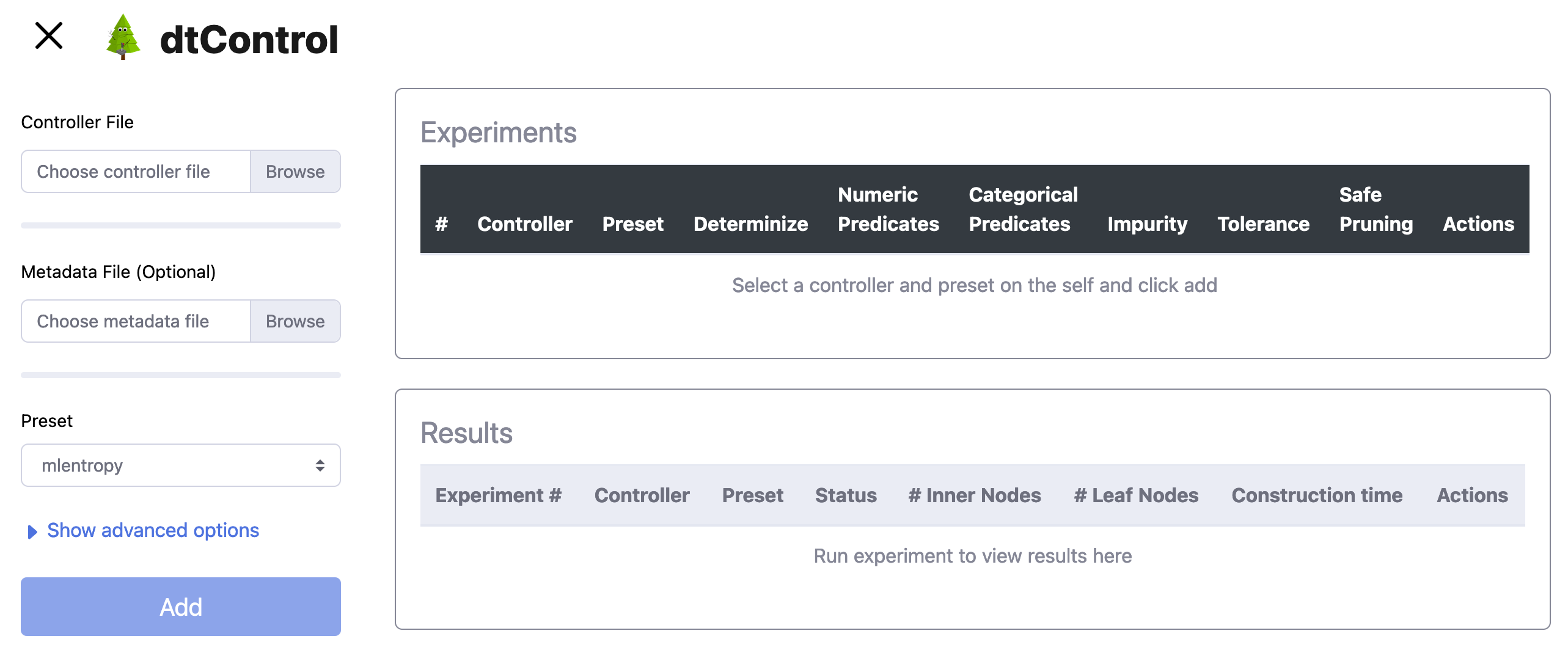
It offers a sidebar for easy selection of the controller file and hyper-parameters, an experiments table where benchmarks can be queued, and a results table in which some statistics (number of nodes, construction time, …) of the run are provided. Moreover, users can click on the ‘eye’ icon in the results table to inspect the built decision tree.

Running your first experiment

1. Select controller file: First, choose a controller file by clicking on the Browse Button within the ‘Controller File’ section. The currently supported file formats can be found in Supported tools. You can choose to download all of our examples from our Gitlab repository via this zip archive. Make sure you unzip all files before selecting them. (Alternatively, you can follow the commands provided in The command-line interface).

2. Optional: Select metadata file. This step is completely optional. If wanted, the user can provide a json file containing metadata for the corresponding controller file. An example file for the 10room model can be found here:

   10rooms metadata

3. Select preset: In this step, the user can choose from various different preset options, presented in the section Presets and configuration files. Furthermore, we introduce two additional presents:

   1. custom, which corresponds to section Configurable options. Upon selection this preset, the advanced options menu automatically expands.

   2. algebraic / user-defined, which is described in more detail in section Algebraic User-Defined Predicates.

4. Add experiment: After selecting both the required controller file and the preset, the user can save this experiment by pressing the Add button. Note that the Add button is only clickable, once both required steps are done.

   

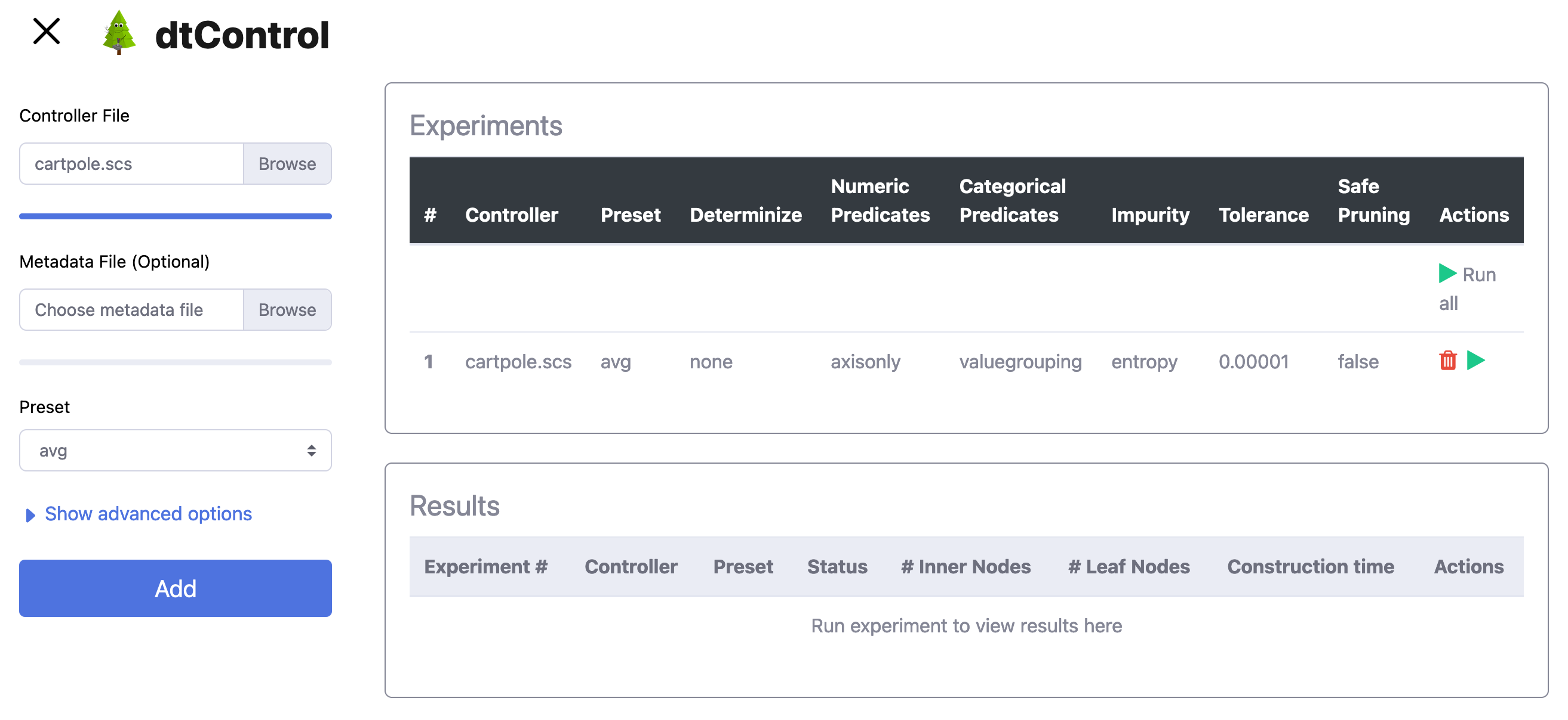
5. Run/ delete experiment: After successfully adding an experiment, the corresponding experiment can be executed by pressing or deleted by pressing . Alternatively, if there are several different experiments, the user can execute all of them by pressing the Run all button.

   

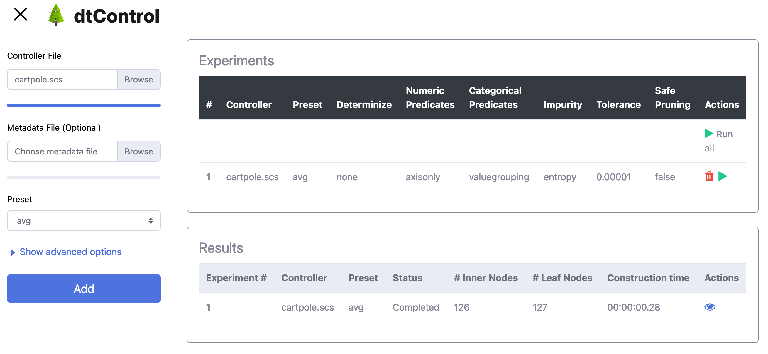
   Once the computation is finished, the experiment will appear in the results section. The experiment can be inspected by clicking . By pressing this button, the user exits the start page and enters the ‘Inspection’ mode.

Inspecting your first result

Select controller file: In order to enter the ‘Inspection’ mode, the user has to click the symbol, within the ‘Results’ section. Upon clicking, a new window will appear where the computed decision tree is displayed.

Inspection mode:

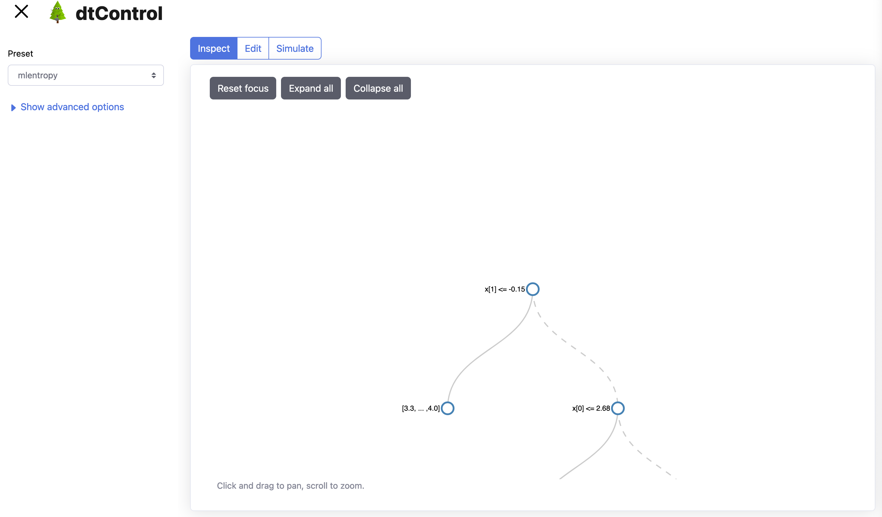
To take a look at the computed decision tree, the user can click and drag to pan and scroll to zoom. By clicking on a node, the node will collapse and absorb all its child nodes. A collapsed node can be simply expanded, by clicking again on it.

Reset focus If you lost the orientation of the root node, simply click on the Reset focus Button to reset the focus on the root node.

Expand all To quickly expand all collapsed nodes, simply click this button.

Collapse all To quickly collapse all nodes within the root node, simply click this button.

Editing your first result

Editing mode: In order to enter the ‘Editing’ mode, the user has to click the Edit Button. At this point the user can either retrain the decision tree from a certain node by clicking on a node and then the Retrain from selected node Button or alternatively start the interactive tree builder from a selected node.

Retrain from selected node Similar to the ‘select preset’ Section in Running your first experiment, the user can can specify the preset used for retraining all child nodes.

Start interactive tree builder from selected node By selecting a node and pressing this button, the user enters the interactive tree builder mode.

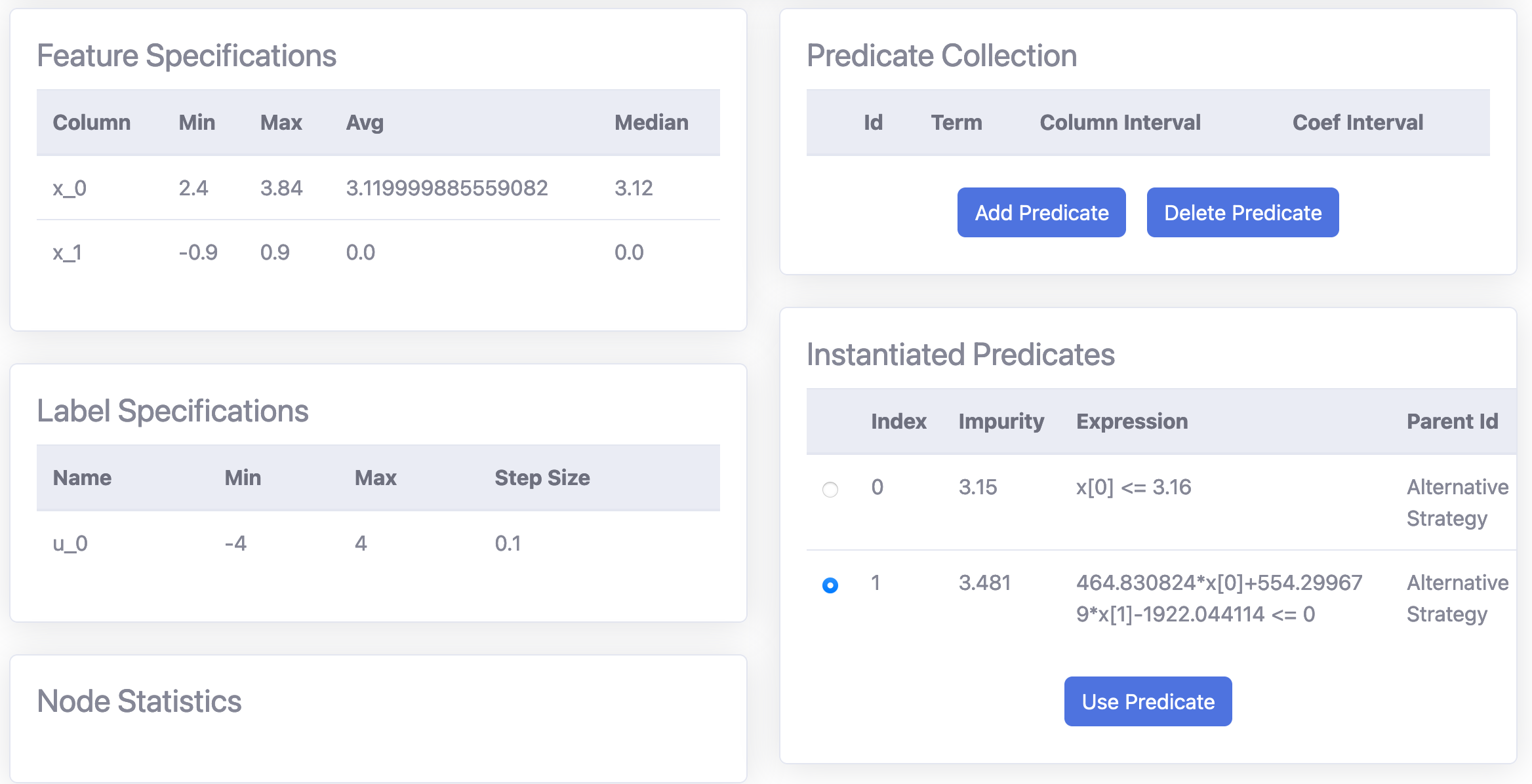
The user can now provide for the selected node, a custom predicate. For this purpose, additional information about the current state of the dataset at the current node is displayed. A user defined predicate can be added by pressing the Add predicate Button. The Syntax is described in the Algebraic User-Defined Predicates section. In the ‘Instantiated Predicates’, the user can now select the wanted predicate. Child nodes containing a inhomogeneous set of labels will be labeled with ‘Not yet homogeneous’. For those nodes, the user can again either decide to use the ‘Retrain from selected node’ functionality or start again the ‘interactive tree builder’.

Simulating your first result

Simulation mode: The simulation mode can be entered by clicking the Simulate Button. To start the simulation, the user has to enter a system dynamics file. For this purpose we provide following two example files:

10rooms dynamics

cartepole dynamics

After the system dynamics file is uploaded, the user can enter some initial values for the simulation task.

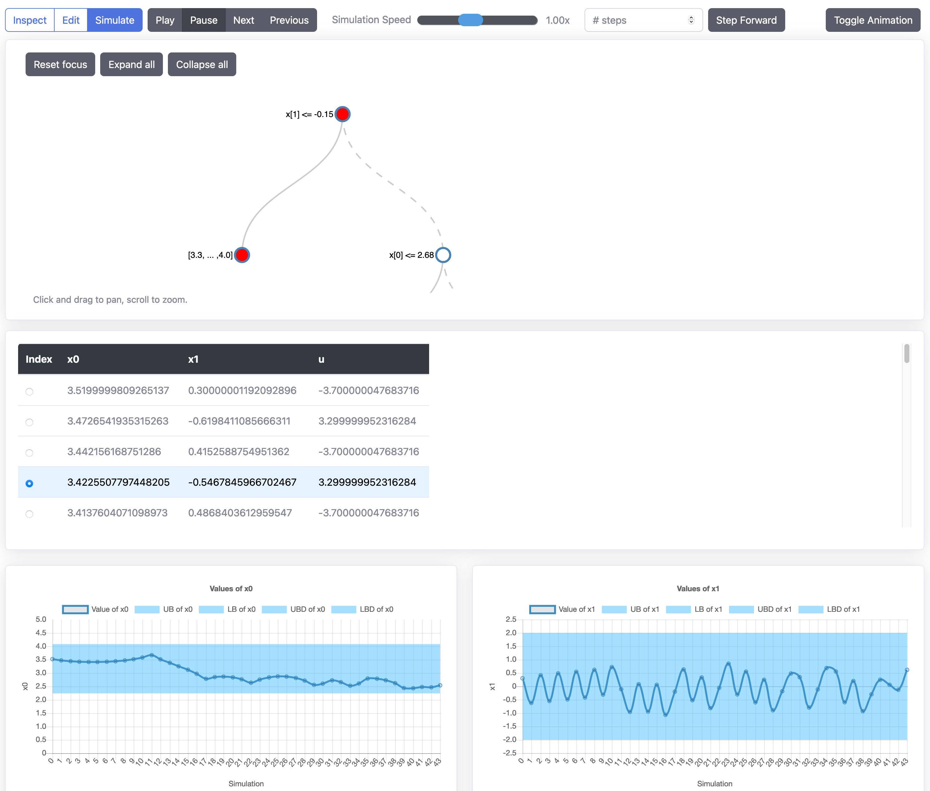
With the buttons Play, Pause, Next and Previous, the user can navigate between the different simulation steps. The corresponding path inside the decision tree, which corresponds to the current simulation values is marked with red nodes.

Semi-automatic Command-Line User Interface

In order the utilize the semi-automatic user interface the user has to import the command-line interface by adding following line to Quick Start with the Python Interface:

from dtcontrol.decision_tree.splitting.context_aware.richer_domain_cli_strategy import RicherDomainCliStrategy

Additionally, create and add the classifier:

cli = RicherDomainCliStrategy(debug=True)

classifiers = [
# Interactive
DecisionTree([cli], Entropy(), 'interactive')
]

After adding these lines of code, the user can follow the commands (which you may copy-paste) from this demonstration video:

Warning

We expect the user to have an activated virtual environment at this point.

Algebraic User-Defined Predicates

The support for algebraic user-defined predicates forms one of the cornerstones of dtControl 2.0. In this subsection we introduce several different extensions for predicates. The most simplified predicate structure can be summarized as follows:

Standard predicate

\[\textit{term} \sim \textit{term}\]

Where \(\textit{term}\) is an arbitrary arithmetic term, using any elementary function that can be parsed by SymPy. \(\sim\) is a standard comparator from the set \(\{\texttt{<=,>=,<,>,=}\}\).

Note

The \(i\) -th feature can be referenced by typing x_i. With \(i \in \mathbb{N}_0\) and x_0 referencing the first feature.

Some arbitrary examples:

Example standard predicate	dtControl syntax
\(x_0 \leq 0.5\)	x_0 <= 0.5
\(x_0 * 12 + x_1 * 3 \ge x_0 * 2 - x_2 * 3\)	x_0 * 12 + x_1 * 3 >= x_0 * 2 - x_2 * 3
\(\sqrt{x_0} * x_2 + log(x_1) - \displaystyle\frac{x_2}{x_3} \leq x_4\)	sqrt(x_0) * x_2 + log(x_1) - (x_2)/(x_3) <= x_4
\(1.0546e-34 + 90 - x_2 \ge x_0\)	1.0546e-34 + 90 - x_2 >= x_0
\(e^{10} + ln(2) + \displaystyle\frac{x_1}{x_2} \ge 0\)	e^10 + ln(2) + (x_1)/(x_2) >= 0
\(sin(cos(12)) + x_2^{x_3} \leq x_1\)	sin(cos(12)) + x_2^(x_3) <= x_1

Coefficient predicates

Coefficients overcome the limitations of standard predicates by enabling the usage of coefficients within \(\textit{term}\). In dtControl 2.0 we distinguish between finite and infinite coefficients.

Finite coefficients: In order to bundle different variations of one single predicate, we introduce finite coefficients. The concept builds upon Standard predicate and can be describes as the following:

\[\textit{term}_f \sim \textit{term}_f \textit{; def}\]

With the extension of \(\textit{term}_f\) being an arbitrary algebraic term using Finite Coefficients defined in \(\textit{def}\). The general idea is to utilize Finite Coefficients \(c_i\) within \(\textit{term}_f\) and extend the finished predicate with a semicolon, followed by the concrete coefficient definition \(C_i \subseteq \mathbb{R}\) with \(c_i \in C_i\).

Note

For computational reasons, the only restriction we insist on is \(|C_i| \in \mathbb{N}\). However, it should be noted that specifying too many or too large sets results in an infeasibly large set of predicates.

Some arbitrary examples:

Example finite coefficient predicate	dtControl syntax
\(\sqrt{x_0} * c_0 + log(x_1) - \displaystyle\frac{x_2}{c_1} \leq c_2 \text{; }c_0 \in \{-\frac{1}{3},\frac{1}{3}\} \text{; } c_1 \in \{1,2\} \text{; } c_2 \in \{\sqrt{2}, \pi\}\)	sqrt(x_0) * c_0 + log(x_1) - (x_2 / c_1) <= c_2; c_0 in {-(1/3),(1/3)}; c_1 in {1, 2}; c_2 in {sqrt(2), pi}
\(1.0546e-34 + 90 - c_0 \ge x_0 \text{; }c_0 \in \{0,12\}\)	1.0546e-34 + 90 - c_0 >= x_0; c_0 in {0,12}
\(e^{10} + ln(2) + \displaystyle\frac{x_2}{c_0} \ge 0 \text{; }c_0 \in \{-\frac{1}{9},\frac{2}{3}\}\)	e^10 + ln(2) + (x_2 / c_0) >= 0; c_0 in {-(1/9), (2/3)}
\(sin(cos(12)) + c_0^{c_1} \leq x_1 \text{; }c_0 \in \{1,2,3\} \text{; } c_1 \in \{4\}\)	sin(cos(12)) + c_0^(c_1) <= x_1; c_0 in {1,2,3}; c_1 in{4}

Infinite coefficients: Infinite coefficients extend the concept of finite coefficients and enable the usage of more generic terms. Building upon the structure of Finite Coefficients, predicates using infinite coefficients can be described as the following:

\[\textit{term}_i \sim \textit{term}_i\]

With the extension of \(\textit{term}_i\) being an arbitrary algebraic term using infinite coefficients. Infinite coefficients can be used throughout the term without defining them. dtControl 2.0 uses SciPy to heuristically determine their exact substituted value.

Note

The difference between infinite and finite coefficients is that latter need a concrete definition whereas infinite coefficients can be seen as a placeholder for ‘perfect’-fitting value.

Warning

It should be avoided to combine too many finite and infinite coefficients together as that can easily end up in a combinatorial explosion.

Example: The following predicate \(x_1 * c_0 >= c_1\text{; }c_0 \in \{1,2\}\text{; }c_1 \in \{1,2,3\}\) bundles 6 predicates together.

1. \(x_1 * 1 >= 1\)

2. \(x_1 * 1 >= 2\)

3. \(x_1 * 1 >= 3\)

4. \(x_1 * 2 >= 1\)

5. \(x_1 * 2 >= 2\)

6. \(x_1 * 2 >= 3\)

Feature constraints

The concept of Feature Constraints is provided for explicit situations where the usage of a predicate is only valid under certain constraints within the current controller file. Similar to the previous sections of coefficient predicates, predicates using Feature Constraints can be described as the following:

\[\textit{term}_i \sim \textit{term}_i \textit{; def}_f\]

With the extension of \(\textit{def}_f\) containing the explicit feature constraints. Similar to the finite coefficients, the user can specify the valid range with a by declaring a set with accepted values. Additionally, we also enabled the usage of infinite sets by declaring an interval of the structure [a,b), [a,b], (a,b) or (a,b] with \(a,b \in \mathbb{R}\cup \{-\infty, \infty\}\). To utilize \(\infty\) simply type Inf, infinity or oo. Additionally, we support the possibility to union several different sets by using the keywords or or u.

Note

\((a,b) = \{ x \in \mathbb{R} | a < x < b\}\)

\([a,b) = \{ x \in \mathbb{R} | a \leq x < b\}\)

\((a,b] = \{ x \in \mathbb{R} | a < x \leq b\}\)

\([a,b] = \{ x \in \mathbb{R} | a \leq x \leq b\}\)

Some arbitrary examples:

Example predicates with finite feature constraints	dtControl syntax
\(x_0 \leq 0.5 \text{; }x_0 \in \{1,2,3,\displaystyle\frac{1}{3}\}\)	x_0 <= 0.5; x_0 in {1,2,3,1/3}
\(x_0 + x_1 \leq 3.9 \text{; }x_0 \in \{\displaystyle\frac{1}{3}\}; x_1 \in [1,2) \cup (-\infty,-123]\)	x_0 <= 0.5; x_0 in {1/3}; x_1 in [1,2) or (-Inf,-123]
\(\sqrt{x_0} * c_0 + log(x_1) \geq x_2 * c_1\text{; }x_0 \in \{ \pi \}; x_1 \in [\sqrt{2},\infty); c_0 \in \{1,2,\pi \}; x_1 \in \{1,2\}\)	sqrt(x_0) * c_0 + log(x_1) >= x_2 * c_1; x_0 in {pi}; x_1 in [sqrt(2),Inf); c_0 in {1,2,pi}; x_1 in {1,2}